
New features
For more feasibility of our platform, ALGOGENE now supports new features:
- import multiple custom data files
- specify user-defined file formats
- include user data for backtest
This article provides a stepwise example to demonstrate how to perform these tasks on ALGOGENE platform.
Data Preparation
Suppose we are interested to conduct research on several stocks that are currently not available on ALGOGENE. We downloaded the market data from Yahoo Finance.
For example, we downloaded the daily prices of 2020 for
- 0005.HK, the stock price of HSBC listed on HKEx (https://finance.yahoo.com/quote/0005.HK/history?p=0005.HK)
- 0939.HK, the stock price of China Construction Bank listed on HKEx (https://finance.yahoo.com/quote/0939.HK/history?p=0939.HK)
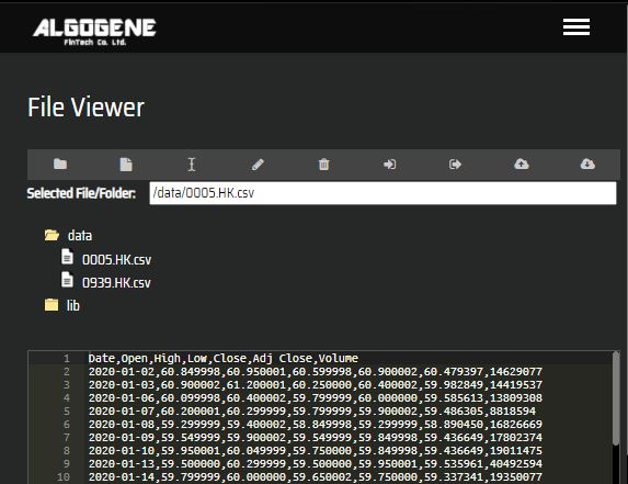
The downloaded files from Yahoo Finance are in csv format. When we open the files using Notepad or other plain text editors, we can see the data structure as follows:
1 2 3 4 5 6 7 8 9 10 | Date,Open,High,Low,Close,Adj Close,Volume 2020-01-02,60.849998,60.950001,60.599998,60.900002,60.479397,14629077 2020-01-03,60.900002,61.200001,60.250000,60.400002,59.982849,14419537 2020-01-06,60.099998,60.400002,59.799999,60.000000,59.585613,13809308 2020-01-07,60.200001,60.299999,59.799999,59.900002,59.486305,8818594 2020-01-08,59.299999,59.400002,58.849998,59.299999,58.890450,16826669 2020-01-09,59.549999,59.900002,59.549999,59.849998,59.436649,17802374 2020-01-10,59.950001,60.049999,59.750000,59.849998,59.436649,19011475 2020-01-13,59.500000,60.299999,59.500000,59.950001,59.535961,40492594 ... |
1 2 3 4 5 6 7 8 9 10 | Date,Open,High,Low,Close,Adj Close,Volume 2020-01-02,6.730000,6.830000,6.730000,6.800000,6.420695,239292513 2020-01-03,6.830000,6.850000,6.720000,6.720000,6.345157,277420033 2020-01-06,6.700000,6.710000,6.580000,6.650000,6.279061,260518248 2020-01-07,6.640000,6.700000,6.600000,6.610000,6.241293,204806676 2020-01-08,6.540000,6.590000,6.480000,6.560000,6.194082,267421237 2020-01-09,6.650000,6.710000,6.600000,6.670000,6.297946,215859440 2020-01-10,6.730000,6.750000,6.680000,6.720000,6.345157,223748680 2020-01-13,6.740000,6.830000,6.740000,6.800000,6.420695,481124394 ... |
As we can see, the files contains 7 columns in total and structured below.
| Column Index | Column Name | Data Type |
|---|---|---|
| 0 | Date | in format of YYYY-MM-DD |
| 1 | Open | float |
| 2 | High | float |
| 3 | Low | float |
| 4 | Close | float |
| 5 | Adj Close | float |
| 6 | Volume | integer |
Data Import
Now, let's import our data files as follows:
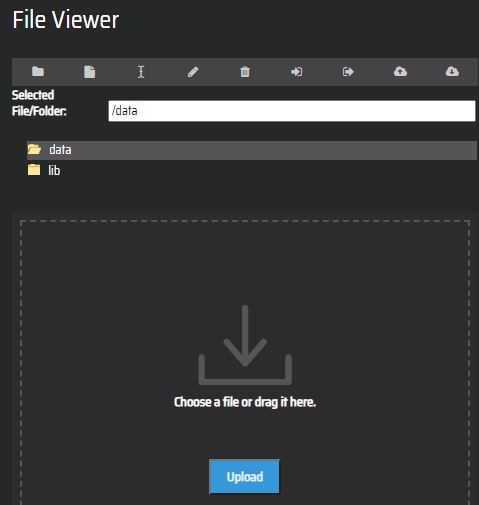
- After login the portal, go to [My History] > [Custom File Viewer]
- Select '/data' directory, then upload data files
- We can then 'Edit' to view the uploaded content
- Now, we need to create a meta file '_meta_.json' to instruct the system how to process the data files.
- '_meta_.json' is in JSON format where we can specify the instrument name in the first key
- in this example, we label them as '0005.HK' and '0939.HK' respectively
- it should be noticed that our specified name has to be distinct from ALGOGENE's existing instruments. Otherwise, the system will skip processing our data files.
- the second key of '_meta_.json' should contain the following
- 'file': the file name on the cloud directory
- 'file_delimiter': the file delimiter used in a data file
- 'period_start': the starting date of a data file, in the format of YYYY-MM-DD
- 'period_end': the end date of a data file, in the format of YYYY-MM-DD
- 'settleCurrency': the settlement currency of the instrument (it is HKD in our example)
- 'contractSize': the number of share per each lot of the instrument
- 'fmt_time': specified the date format in a data file, in Python date encoding
- %Y: the year in four-digit format, eg. "2018"
- %y: the year in two-digit format, that is, without the century. For example, "18" instead of "2018"
- %m: the month in 2-digit format, from 01 to 12
- %b: the first three characters of the month name. eg. "Sep"
- %d: day of the month, from 1 to 31
- %H: the hour, from 0 to 23
- %M: the minute, from 00 to 59
- %S: the second, from 00 to 59
- %f: the microsecond from 000000 to 999999
- %Z: the timezone
- %z: UTC offset
- %j: the number of the day in the year, from 001 to 366
- %W: the week number of the year, from 00 to 53, with Monday being counted as the first day of the week
- %U: the week number of the year, from 00 to 53, with Sunday counted as the first day of each week
- %a: the first three characters of the weekday, e.g. Wed
- %A: the full name of the weekday, e.g. Wednesday
- %B: the full name of the month, e.g. September
- %w: the weekday as a number, from 0 to 6, with Sunday being 0
- %p: AM/PM for time
- 'col_time': the column position of data date (first column index = 0)
- 'col_open': the column position of open price (first column index = 0)
- 'col_high': the column position of high price (first column index = 0)
- 'col_low': the column position of low price (first column index = 0)
- 'col_close': the column position of closing price (first column index = 0)
- 'col_volume': the column position of volume (first column index = 0)
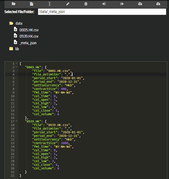
The sample meta file used in the example can be copied here:
1 2 3 4 5 6 7 8 9 10 11 12 13 14 15 16 17 18 19 20 21 22 23 24 25 26 27 28 29 30 31 32 | {
"0005.HK": {
"file": "0005.HK.csv",
"file_delimiter": ",",
"period_start": "2020-01-01",
"period_end": "2020-12-31",
"settleCurrency": "HKD",
"contractSize": 400,
"fmt_time": "%Y-%m-%d",
"col_time": 0,
"col_open": 1,
"col_high": 2,
"col_low": 3,
"col_close": 5,
"col_volume": 6
},
"0939.HK": {
"file": "0939.HK.csv",
"file_delimiter": ",",
"period_start": "2020-01-01",
"period_end": "2020-12-31",
"settleCurrency": "HKD",
"contractSize": 1000,
"fmt_time": "%Y-%m-%d",
"col_time": 0,
"col_open": 1,
"col_high": 2,
"col_low": 3,
"col_close": 5,
"col_volume": 6
}
}
|
Backtest
After we properly setup the '_meta_.json', we can then include our custom instruments for backtest.
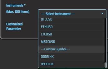
- Go to [Backtest] > [Setting]
- Select '0005.HK' and '0939.HK' in the instrument panel
- 'Start Period' and 'End Period' set to '2020-01' and '2020-12' respectively
- 'Initial Capital' set to 1,000,000
- 'Base Currency' set to 'HKD'
In our example '0005.HK' and '0939.HK', the 2 stocks are both in banking sector. Suppose we found that the 2 companies are correlated and therefore we try to test a pair trading strategy on them! A simple trading idea is as follows:
- Based on a sliding window approach to collect the last 5 closing price
- Fit a simple linear regression model without intercept Y = b*X for the 2 series
- if residual > certain level of the stadard error, buy 1 lot of X and sell b lot of Y
- if residual < -1* certain level of the stadard error, sell 1 lot of X and buy b lot of Y
- for any opened pair, close the position 5 day later
The full source code can be referred below:
1 2 3 4 5 6 7 8 9 10 11 12 13 14 15 16 17 18 19 20 21 22 23 24 25 26 27 28 29 30 31 32 33 34 35 36 37 38 39 40 41 42 43 44 45 46 47 48 49 50 51 52 53 54 55 56 57 58 59 60 61 62 63 64 65 66 67 68 69 70 71 72 73 74 75 76 77 78 79 | from AlgoAPI import AlgoAPIUtil, AlgoAPI_Backtest from datetime import datetime, timedelta import statsmodels.api as sm class AlgoEvent: def __init__(self): self.lasttradetime = datetime(2000,1,1) self.orderPairCnt = 0 self.arrSize = 5 self.arr_closeY = [] self.arr_closeX = [] def start(self, mEvt): self.myinstrument_Y = mEvt['subscribeList'][0] self.myinstrument_X = mEvt['subscribeList'][1] self.evt = AlgoAPI_Backtest.AlgoEvtHandler(self, mEvt) self.evt.start() def on_bulkdatafeed(self, isSync, bd, ab): if isSync: # check condition for open position if bd[self.myinstrument_Y]['timestamp'] >= self.lasttradetime + timedelta(hours=24): self.lasttradetime = bd[self.myinstrument_Y]['timestamp'] # collect observations self.arr_closeY.append(bd[self.myinstrument_Y]['lastPrice']) self.arr_closeX.append(bd[self.myinstrument_X]['lastPrice']) # kick out the oldest observation if array size is too long if len(self.arr_closeY)>self.arrSize: self.arr_closeY = self.arr_closeY[-self.arrSize:] if len(self.arr_closeX)>self.arrSize: self.arr_closeX = self.arr_closeX[-self.arrSize:] # fit linear regression Y = self.arr_closeY X = self.arr_closeX #X = sm.add_constant(X) #add this line if you want to include intercept in the regression model = sm.OLS(Y, X) results = model.fit() self.evt.consoleLog(results.summary()) coeff_b, tvalue, mse = results.params[-1], results.tvalues, results.mse_resid # compute current residual, e = Y - b*X diff = self.arr_closeY[-1] - coeff_b*self.arr_closeX[-1] if diff>0.1*mse: # regard Y as overpriced, X as underpriced self.orderPairCnt += 1 self.openOrder(-1, self.myinstrument_Y, self.orderPairCnt, 1) #short Y if coeff_b>0: self.openOrder(1, self.myinstrument_X, self.orderPairCnt, abs(round(coeff_b,2))) #long X else: self.openOrder(-1, self.myinstrument_X, self.orderPairCnt, abs(round(coeff_b,2))) #short X elif diff<-0.1*mse: # regard Y as underpriced, X as overpriced self.orderPairCnt += 1 self.openOrder(1, self.myinstrument_Y, self.orderPairCnt, 1) #long Y if coeff_b>0: self.openOrder(-1, self.myinstrument_X, self.orderPairCnt, abs(round(coeff_b,2))) #short X else: self.openOrder(1, self.myinstrument_X, self.orderPairCnt, abs(round(coeff_b,2))) #long X def openOrder(self, buysell, instrument, orderRef, volume): order = AlgoAPIUtil.OrderObject() order.instrument = instrument order.orderRef = orderRef order.volume = volume order.openclose = 'open' order.buysell = buysell order.ordertype = 0 #0=market_order, 1=limit_order order.holdtime = self.arrSize*24*60*60 #unit in second self.evt.sendOrder(order) def on_marketdatafeed(self, md, ab): pass def on_orderfeed(self, of): pass def on_dailyPLfeed(self, pl): pass def on_openPositionfeed(self, op, oo, uo): pass |
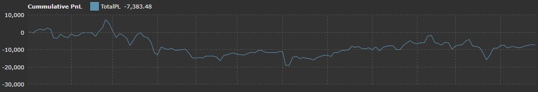
The backtest result can be generated as usual.
Demo Video
Now, you learnt how to plugin your own data files on the platform. Try backtest with a custom dataset today! Happy Trading!

