In the dynamic world of trading, having a robust strategy is paramount for success. Whether you're a seasoned quant trader or new to the field, understanding various trading styles, theories, and models is essential. This blog will dissect trading strategies, elaborate on basic mathematical concepts behind them, and provide practical examples for better comprehension.

Trading Styles

Trading strategies can broadly be classified into four primary styles:

1. Scalping

• Holding Period: Milliseconds to minutes
• Objective: Capture small price changes for quick profits.
• Example: A scalper might enter a position in a liquid stock like Apple (AAPL) and aim for a profit of $0.10 per share, executing multiple trades throughout the day to accumulate profits.

2. Day Trading

• Holding Period: Intraday, all positions closed before market close.
• Objective: Take advantage of short-term price movements.
• Example: If you buy 100 shares of Tesla (TSLA) at $700 and sell them at $710 by end of day, your profit would be $1,000 (100 shares × $10 gain).

3. Swing Trading

• Holding Period: Several days to weeks.
• Objective: Capture larger price movements by holding positions through price fluctuations.
• Example: Buying a stock at $50 and holding it until it reaches $60 over a week could yield a $1,000 profit on 100 shares.

4. Position Trading

• Holding Period: Months to years.
• Objective: Long-term investment strategy.
• Example: Purchasing shares of Amazon (AMZN) at $1,500 and holding them for two years until they rise to $3,000, yielding significant long-term returns.

Investment & Trading Theories

1. Fundamental Analysis (FA)

Fundamental analysis examines economic and financial factors influencing a security's value. Key areas include:

• Macroeconomic Indicators: GDP, interest rates, unemployment rates.
• Microeconomic Factors: Company management, financial statements, and growth potential.

2. Technical Analysis (TA)

It based on the assumption that history will repeat itself and the financial market is sufficiently efficient. A security's price mostly reflects all available information, and therefore analysing past price and volume movements can predict future market behavior. Common tools include:

• Candlestick Charts

  Indicate historical patterns through price trends and potential reversals.

• Moving Averages

  Smooth out price data to help identify trends. For example, if a stock's moving average crosses above another, it could signal a potential buy.

• Oscillator Indicators

  indicators that fluctuate within a specific range, helping traders identify overbought or oversold conditions in the market.

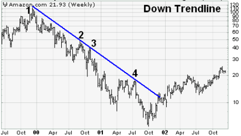
• Support and Resistance Levels

  Key price points on a chart where an asset tends to stop and reverse direction.

  • Support refers to a price level where buying interest is strong enough to prevent the price from falling further
  • resistance is where selling interest is sufficient to cap price increases

Typical technical patterns include:

• Trending - sometimes called 'bulls' for an uptrend, and 'bears' for a downtrend


• Mean Reverting
• Momentum
• Breakout
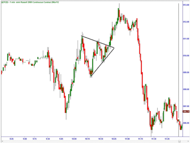
• Pennants - two trendlines that eventually converge


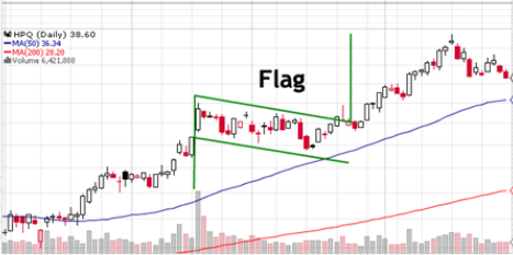
• Flags - two parallel trendlines that can slope up, down or horizontally


• Head and Shoulders

3. Quantitative Analysis and Algorithmic Trading

Quantitative Analysis (QA) focuses on using mathematical and statistical techniques to analyze financial markets and securities. In the context of algorithmic trading, this involves the creation of automated systems that can execute trades based on predefined criteria, leveraging historical data and quantitative models for optimal decision-making.

Quantitative traders utilize advanced mathematical models to identify trading opportunities. These models can incorporate various statistical techniques, such as:

• Regression Analysis: Used to determine relationships between variables. For example, a multiple linear regression model could assess how well economic indicators (like interest rates and GDP) can predict stock prices.
• Stochastic Calculus: Involves modeling the random behaviors in markets, often applied in derivative pricing via models like the Black-Scholes formula.
• Time Series Analysis: Focuses on analyzing historical price data to identify patterns or trends that can predict future movements.

Formulating and Automating Trading Strategies

One of the primary goals of quantitative analysis is to develop and automate trading strategies. This involves several key steps:

1. Strategy Development: Formulate a strategy based on research and data analysis. For instance, you may discover that a certain stock historically tends to rise after a specific type of news release.
2. Backtesting: Before deploying a strategy in live markets, it is crucial to backtest using historical data to assess its effectiveness. Backtesting involves simulating trades using past market conditions to evaluate potential profitability or risk.
3. Execution: Once the strategy is validated, it’s implemented through an algorithm that can execute trades automatically based on the predetermined conditions.

Data Inputs for Quantitative Analysis

Quantitative trading systems can harness a wide variety of data inputs, often broader than traditional Fundamental Analysis (FA) or Technical Analysis (TA):

• Price-Volume Market Data: Historical price and volume data are fundamental to understanding market behavior.
• Economic Statistics: Macroeconomic data such as unemployment rates, interest rates, and GDP can be crucial indicators.
• Company Earnings: Earnings reports and other corporate announcements often lead to significant price movements.
• News and Social Media Sentiment: Analyzing news articles or social media trends can offer insights into market sentiment and influence trading decisions.
• Weather Patterns: Particularly relevant for commodities, as weather can impact supply and demand.

Classification of Trading Strategy

1. Rule-Based/ Deterministic

• Precisely defines a trade set-up, eg.
• exactly how much money will be placed on each trade (position size)
• exactly what the risk and profit will be (stop-loss, take-profit level)
• exactly the set of financial instruments will be applied to (specific sector)
• Examples:
• A fundamental analyst may regard a company as "good to buy" if it meets the following conditions.
• Debt-to-Asset ratio less than 40%, AND
• Net Income for the past 3 years are positive, AND
• Profit margin is above 1%.

2. Subjective/ Dynamic

• Usually event driven and sometimes involve human judgement
• "guideline" based rather than a set of fixed rules, could be adaptable to changing market conditions, eg.
• Switch trading model according to different market scenario
• Dynamic Delta hedging for options portfolio
• Rebalancing stock weights in a portfolio
• Determine the hedge ratio in a static pair trading
• Examples:
• Dynamic Pair Trading

Suppose there are 50 stocks from the same Technology sectors. From which, you can construct ₅₀C₂ = 1225 pairs in total. Now, you perform the modelling process as follows

1. compute the correlation for each pair of stocks
2. identify the pair that have the highest correlation (say X and Y)
3. fit a zero-intercept regression model: Y = βX + ∊
4. if ∊>0, you buy β share of X, and short sell 1 share of Y; otherwise, you short sell β share of X, and buy 1 share of Y
5. Repeat above process regularly (say every month)

In this example, you do not explicitly specify a trading pair at the beginning. Instead, it is derived from a "guideline" of "maximum correlation".

Common Quantitative Strategies & Trading Models

A robust trading model reduces complex systems into quantifiable rules. Below are several common models:

1. Time Series Analysis (ARIMA)

It models the relationship between a security price series {y_t} and its historical prices {y_t-1, ..., y_t-p}, and then based on the formula to forecast the future price movements.

Formula:

y_t = φ₁y_t-1 + ... + φ_py_t-p + ∊_t + ϑ₁∊_t-1 + ... + ϑ_qy_t-q

2. Multiple Linear Regression

It models the relationship between a security {y_t} and other variables {x_1,t, ... , x_p,t}, which could either be tradable (eg. other stocks) or non-tradable (eg. GDP) variables. This model could be used to estimate the "theoretical fair" value of Y, and then to evaluate whether the current price level is "cheap" to buy.

Formula:

y_t = β₀ + β₁X₁ + ... + β_pX_p + ∊_t

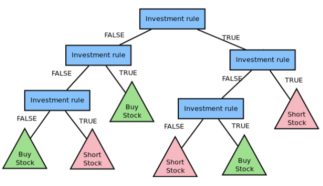
3. Decision Trees

A flowchart structure that breaks down decisions and outcomes, useful for complex trading strategies.

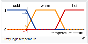
4. Fuzzy logic

This model is widely used to handle the concept of partial truth, and have the capability of interpreting data and information that are vague and lack certainty. It enables all data inputs feed into the fuzzy membership functions subject to proper data transformation, and then output a value spectrum ranging from 0 to 1.

From financial market perspective, one can interpret and transform the output as the probability of "Buy", "Hold", and "Sell" signal.

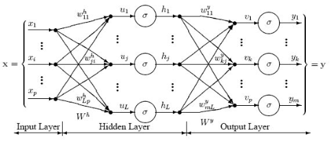
5. Neural Network

This model aims to predict price movements through layers of interconnected nodes, mimicking human brain functionality. It can tackle 2 problems:

1. forecast exactly close price or return next day
2. binary classification (price will go up or down)

For (i), it can be achieved by regressing {Y_(t+1)} to {Y_t} by minimizing the mean-squared-error of the price difference. For (ii), it can also be achieved by applying a softmax function at the output layer to convert the output value into [0,1].

Trading Strategy/Model Parameters

A trading strategy can range from a straightforward one-line formula to a complex deep network topology. There are numerous ways to design and implement features in a trading strategy, allowing researchers to customize and combine various techniques for model building. Given the vast array of parameters that can be utilized in trading, it's challenging to list them all comprehensively. Below, we provide a categorization of some commonly used parameters for inspiration.

1. Trading Parameters

• Order Entry
• Market Open - to determine if instrument can be traded on a particular exchange at a particular time
• Market Liquidity Spread - a way to determine if it is "easy" to transact without large price discount, usually represent in half-spread, i.e. 0.5*(ask price - bid price)/(mid price)
• Market Transaction Volume - a way to determine if it is "easy" to transact without large impact on market price movement
• Market Order Book - a way to determine the market depth if it is "easy" to transact without large impact on market price movement
• Outstanding Inventory - a way to determine if your portfolio is too concentrated on a particular security
• Order Size - for better capital management, one might scale up the trade volume when portfolio value increase
• Order Exit
• Market Volatility - a way to determine the market sentiment in response to unexpected/unfavor events
• Holding Period - to exit a trade where the previous trade signal expired
• Take Profit Level - a way to close out a position as soon as it achieve a target profit, usually represent as a percentage of the order entry price
• Stop Loss Level - a risk management measure to cap your potential loss below a certain level, usually represent as a percentage of the order entry price
• Trailing Stop Loss Level - a severe risk management measure to close out all portfolio positions and to cap your total loss below such level, usually represent as a percentage of the initial portfolio value
• Order Size - to exit a trade with partial or fully close out

2. Model Parameters

• General:
• Sampling Size - the number of observations used for model building, a statistical rule of thumb for 30 observations per model parameter
• Variable List - the number of variables used for model building, could be singleton, multivariate, independent, or auto-regressive, depending on user design, model nature and available datasets
• Data Frequency - the frequency of observations used for model building, could be daily, monthly, or annual data depending on available datasets and trading horizon
• Calibration Frequency - the frequency to update/ re-train/ re-build a model, could be hourly, daily, or monthly, depending on available datasets and trading horizon
• Specific:
• Auto-Regressive Model

Take AR(1) as an example, the model parameter Φ₁ could provide insights about the current market status. In general,

y_t = c + φ₁y_t-1 + ∊_t

• If Φ₁ > 1, {y_t} is in an upward trending
• If Φ₁ < -1, {y_t} is in a downward trending
• If Φ₁ in (-1, 1), {y_t} is mean-reverting


• Multiple Linear Regression

Y = β₀ + β₁X₁ + β₂X₂ + ∊_t

Suppose we regress stock Y with another 2 stocks {X₁,X₂}, the model coefficients {β₁,β₂} could be taken as the hedge ratios in order to construct a delta-neutral portfolio.



• Neural Network

The calibrated coefficients at input layer can be rescale to interpret as the corresponding sensitivity or importance of the input variables {X₁,…,X_p} to stock Y.

Quantitative Analysis and Algorithmic Trading are essential tools in a trader’s arsenal. By leveraging mathematical computations, extensive datasets, and automated execution, traders can identify, develop, and implement groundbreaking strategies. With the ability to backtest and optimize strategies, traders can enhance their decision-making process, ultimately paving the way for more informed and profitable trading.

Introducing ALGOGENE's Powerful Backtest Engine

At ALGOGENE, we understand the pivotal role that robust testing plays in developing successful trading strategies. Our High-speed Backtest Engine is designed to empower traders of all levels, providing an intuitive, event-driven architecture that supports both historical backtesting and real-time simulation.

With over 20 years of full tick history across a variety of asset classes—including stocks, cryptocurrencies, and forex—you can dive deep into the nuances of market behavior. Our cloud-based development environment is equipped with mainstream Python libraries, making it easy to craft and evaluate algorithms without the hassle of local setup.

One of the standout features of our platform is the AI/ML capabilities, which allow you to input your ideas and have our artificial intelligence generate potential strategies for you. This means that whether you're a seasoned quant or just getting started, you can explore innovative approaches with relative ease.

Plus, with one-click live deployment, you can seamlessly connect to over 30 global exchanges, ensuring a smooth transition from testing to real-world trading. At ALGOGENE, we aim to provide you with the tools necessary to refine your strategies and gain confidence in your trades, all backed by enterprise-level security to protect your data assets. Join us in taking your trading journey to the next level!