
What is Average True Range?
The Average True Range is a technical analysis indicator, originally developed by J. Welles Wilder. ATR does not provide indication about price trend. Instead, it measures the market volatility for a given period N. A common choice of N would be 14.
Calculation
The range of a trading day is simply measured as High - Low. A True Range extends the definition to take into account of yesterday's closing price, which is taken as the maximum of:
- current period's high minus the current period's low;
- the absolute value of the current period's high minus the previous close; and
- the absolute value of the current period's low minus the previous close
Mathematically, true range on day t is calculated as
which can be simplified to:
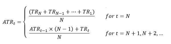
Now, taking the average of {TRt} will produce ATR. There are 2 common forms of ATR.
- Simple Moving Average ATR
- Exponential Moving Average ATR
Interpretation
ATR is simple to calculate and only needs historical price data. It is used primarily to measure volatility caused by gaps or up/ down moves. A stock experiencing a high level of volatility will have a higher ATR, while low market volatility will result in a lower ATR. However, as ATR calculated for a particular stock simply measures its own range of price movement over a period, its value is not comparable to other stocks.
The ATR is commonly used as an exit method. For example, if a trader observe the current ATR increase significantly from the previous value, it probably means the market is highly fluctuating and therefore, the trader could unwind some of his positions to reduce the risk.
ATR sometimes can be used for position sizing for order entry. For example, current ATR value (or a multiple of it) can be used as the stop-loss distance when calculating the trade volume based on trader's risk tolerance. In this case, ATR provides a dynamic risk limit dependent on the market volatility.
Limitation
There are several limitations for ATR indicator.
- ATR only measures volatility and not the direction of price trend, which can sometimes result in mixed signals, particularly when markets are experiencing pivots or when trends are at turning points.
- ATR is a subjective measure. There is no reference point telling you whether the current market is volatile or not. ATR should always be compared against earlier values to get a feel of a trend's strength or weakness.
Implementation
There is a technical analysis python package 'ta-lib' that provides the EMA form of ATR computation.
1 2 3 4 5 6 7 | from talib import ATR arrHigh = [...] arrLow = [...] arrClose = [...] arrATR = ATR(arrHigh, arrLow, arrClose, _period) |
On the other hand, as the formula is fairly simple, we can also code on our own.
1 2 3 4 5 6 7 8 9 10 11 12 13 14 15 16 17 | def my_ATR(obs,n): _n = len(obs) if _n<n: return [] arrTR = [None]*_n arrATR = [None]*_n i = 0 last_k = None for k in obs: if last_k!=None: arrTR[i] = max(k["h"], last_k["c"]) - min(k["l"], last_k["c"]) last_k = k i+=1 arrATR[n] = sum(arrTR[1:n+1])/float(n) for i in range(n+1,_n): arrATR[i] = (arrATR[i-1]*(n-1) + arrTR[i])/float(n) return arrATR |
Example
Suppose we have collected below 50 candle observations.
1 2 3 4 5 6 7 8 9 10 11 12 13 14 15 16 17 18 19 20 21 22 23 24 25 26 27 28 29 30 31 32 33 34 35 36 37 38 39 40 41 42 43 44 45 46 47 48 49 50 51 52 | [
{"t":"2021-04-21", "o":29451.15, "h":29342.311, "l":28692.311, "c":28953.55},
{"t":"2021-04-22", "o":28953.55, "h":29233.099, "l":28719.85, "c":28670.75},
{"t":"2021-04-23", "o":28670.75, "h":28774.158, "l":28468.75, "c":28724.45},
{"t":"2021-04-24", "o":28724.45, "h":28819, "l":28547.852, "c":28732.65},
{"t":"2021-04-27", "o":28732.65, "h":29213.1, "l":28711.793, "c":29099.35},
{"t":"2021-04-28", "o":29099.35, "h":29250.599, "l":28711.793, "c":28832.35},
{"t":"2021-04-29", "o":28832.35, "h":29051.646, "l":28806.593, "c":28913.85},
{"t":"2021-04-30", "o":28913.85, "h":29137.311, "l":28854.35, "c":29185.452},
{"t":"2021-05-01", "o":29185.452, "h":29418.111, "l":29064.505, "c":29171.652},
{"t":"2021-05-03", "o":29171.652, "h":28685.6, "l":28685.6, "c":28685.6},
{"t":"2021-05-04", "o":28685.6, "h":28700, "l":28678.45, "c":28697},
{"t":"2021-05-05", "o":28697, "h":28712.05, "l":28197.617, "c":28408.65},
{"t":"2021-05-06", "o":28408.65, "h":28621.5, "l":28165.705, "c":28415.85},
{"t":"2021-05-07", "o":28415.85, "h":28691.705, "l":28306.15, "c":28541.95},
{"t":"2021-05-08", "o":28541.95, "h":28837.764, "l":28356.65, "c":28707.15},
{"t":"2021-05-11", "o":28707.15, "h":28892.752, "l":28571.65, "c":28814.35},
{"t":"2021-05-12", "o":28814.35, "h":28892.752, "l":28404, "c":28228.45},
{"t":"2021-05-13", "o":28228.45, "h":28295.905, "l":27762.746, "c":27966.1},
{"t":"2021-05-14", "o":27966.1, "h":28212.064, "l":27835.15, "c":27893.85},
{"t":"2021-05-15", "o":27893.85, "h":28052.358, "l":27616.2, "c":27893.05},
{"t":"2021-05-18", "o":27893.05, "h":28245.45, "l":27703.746, "c":28139.85},
{"t":"2021-05-19", "o":28139.85, "h":28289.9, "l":27703.746, "c":28307.55},
{"t":"2021-05-21", "o":28307.55, "h":28635.764, "l":28307.25, "c":28342.15},
{"t":"2021-05-22", "o":28342.15, "h":28635.764, "l":28252.397, "c":28573.95},
{"t":"2021-05-25", "o":28573.95, "h":28620.517, "l":28269.858, "c":28396.95},
{"t":"2021-05-26", "o":28396.95, "h":28620.517, "l":28163.25, "c":28521.85},
{"t":"2021-05-27", "o":28521.85, "h":29015.6, "l":28458.65, "c":29026.25},
{"t":"2021-05-28", "o":29026.25, "h":29261.25, "l":29003.15, "c":29090.75},
{"t":"2021-05-29", "o":29090.75, "h":29251.45, "l":28976.05, "c":29200.65},
{"t":"2021-06-01", "o":29200.65, "h":29378.35, "l":29086.7, "c":29245.35},
{"t":"2021-06-03", "o":29245.35, "h":29451.15, "l":29451.15, "c":29451.15},
{"t":"2021-06-04", "o":29451.15, "h":29537.164, "l":29220.95, "c":29273.45},
{"t":"2021-06-05", "o":29273.45, "h":29400.197, "l":28887.817, "c":28904.95},
{"t":"2021-06-07", "o":28904.95, "h":29095.3, "l":28741.064, "c":29027.9},
{"t":"2021-06-08", "o":29027.9, "h":29095.3, "l":28741.064, "c":29036.8},
{"t":"2021-06-09", "o":29036.8, "h":29040.25, "l":28632.711, "c":28876.15},
{"t":"2021-06-10", "o":28876.15, "h":29015.617, "l":28653.146, "c":28794.2},
{"t":"2021-06-11", "o":28794.2, "h":28901.305, "l":28707.75, "c":28741.8},
{"t":"2021-06-12", "o":28741.8, "h":28987.417, "l":28671.95, "c":28759.95},
{"t":"2021-06-14", "o":28759.95, "h":28999.552, "l":28742.8, "c":28838.5},
{"t":"2021-06-15", "o":28838.5, "h":28999.552, "l":28742.8, "c":28841.9},
{"t":"2021-06-16", "o":28841.9, "h":28891.3, "l":28763.8, "c":28866.3},
{"t":"2021-06-17", "o":28866.3, "h":28986.6, "l":28438.25, "c":28616.8},
{"t":"2021-06-18", "o":28616.8, "h":28649.8, "l":28244.4, "c":28249.8},
{"t":"2021-06-19", "o":28249.8, "h":28630.6, "l":28170.5, "c":28567.85},
{"t":"2021-06-21", "o":28567.85, "h":28853.7, "l":28502.05, "c":28537.7},
{"t":"2021-06-22", "o":28537.7, "h":28853.7, "l":28502.05, "c":28536.7},
{"t":"2021-06-23", "o":28536.7, "h":28670.4, "l":28309, "c":28642.4},
{"t":"2021-06-24", "o":28642.4, "h":28650.4, "l":28236, "c":28425.15},
{"t":"2021-06-25", "o":28425.15, "h":28914.15, "l":28396, "c":28765.65}
]
|
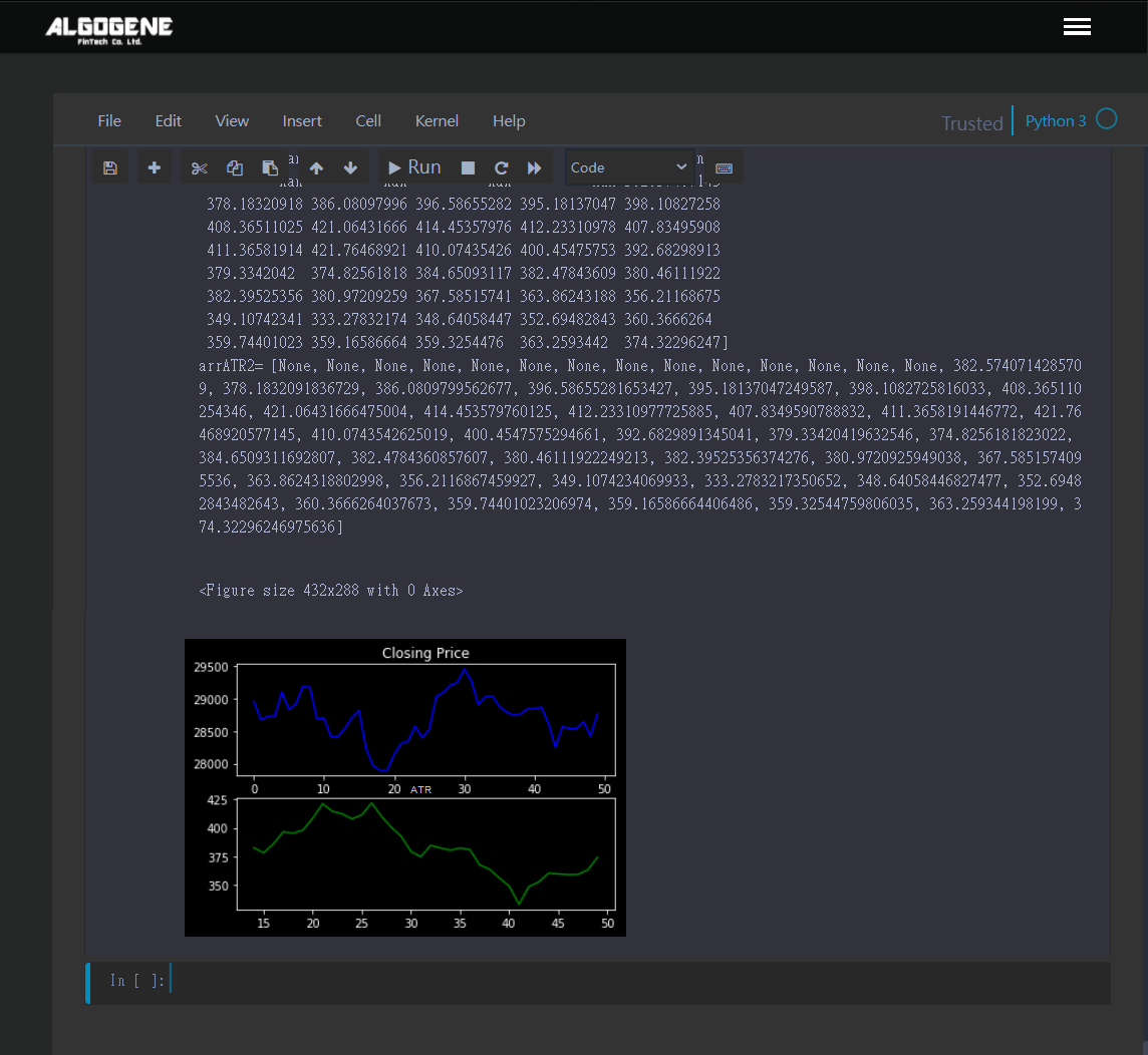
Now, we are interested in calculating a 14-day ATR.
1 2 3 4 5 6 7 8 9 10 11 12 13 14 15 16 17 18 19 20 21 22 23 24 25 26 27 28 29 30 31 32 33 34 35 36 37 38 39 40 41 42 43 44 45 46 47 48 49 50 51 52 53 54 55 56 57 58 59 60 61 62 63 64 65 66 67 68 69 70 71 72 73 74 75 76 77 78 79 80 81 82 83 84 85 86 87 88 89 90 91 92 93 94 95 96 97 98 99 100 101 102 103 104 105 106 107 108 109 | %matplotlib inline import numpy as np from talib import ATR obs = [ {"t":"2021-04-21", "o":29451.15, "h":29342.311, "l":28692.311, "c":28953.55}, {"t":"2021-04-22", "o":28953.55, "h":29233.099, "l":28719.85, "c":28670.75}, {"t":"2021-04-23", "o":28670.75, "h":28774.158, "l":28468.75, "c":28724.45}, {"t":"2021-04-24", "o":28724.45, "h":28819, "l":28547.852, "c":28732.65}, {"t":"2021-04-27", "o":28732.65, "h":29213.1, "l":28711.793, "c":29099.35}, {"t":"2021-04-28", "o":29099.35, "h":29250.599, "l":28711.793, "c":28832.35}, {"t":"2021-04-29", "o":28832.35, "h":29051.646, "l":28806.593, "c":28913.85}, {"t":"2021-04-30", "o":28913.85, "h":29137.311, "l":28854.35, "c":29185.452}, {"t":"2021-05-01", "o":29185.452, "h":29418.111, "l":29064.505, "c":29171.652}, {"t":"2021-05-03", "o":29171.652, "h":28685.6, "l":28685.6, "c":28685.6}, {"t":"2021-05-04", "o":28685.6, "h":28700, "l":28678.45, "c":28697}, {"t":"2021-05-05", "o":28697, "h":28712.05, "l":28197.617, "c":28408.65}, {"t":"2021-05-06", "o":28408.65, "h":28621.5, "l":28165.705, "c":28415.85}, {"t":"2021-05-07", "o":28415.85, "h":28691.705, "l":28306.15, "c":28541.95}, {"t":"2021-05-08", "o":28541.95, "h":28837.764, "l":28356.65, "c":28707.15}, {"t":"2021-05-11", "o":28707.15, "h":28892.752, "l":28571.65, "c":28814.35}, {"t":"2021-05-12", "o":28814.35, "h":28892.752, "l":28404, "c":28228.45}, {"t":"2021-05-13", "o":28228.45, "h":28295.905, "l":27762.746, "c":27966.1}, {"t":"2021-05-14", "o":27966.1, "h":28212.064, "l":27835.15, "c":27893.85}, {"t":"2021-05-15", "o":27893.85, "h":28052.358, "l":27616.2, "c":27893.05}, {"t":"2021-05-18", "o":27893.05, "h":28245.45, "l":27703.746, "c":28139.85}, {"t":"2021-05-19", "o":28139.85, "h":28289.9, "l":27703.746, "c":28307.55}, {"t":"2021-05-21", "o":28307.55, "h":28635.764, "l":28307.25, "c":28342.15}, {"t":"2021-05-22", "o":28342.15, "h":28635.764, "l":28252.397, "c":28573.95}, {"t":"2021-05-25", "o":28573.95, "h":28620.517, "l":28269.858, "c":28396.95}, {"t":"2021-05-26", "o":28396.95, "h":28620.517, "l":28163.25, "c":28521.85}, {"t":"2021-05-27", "o":28521.85, "h":29015.6, "l":28458.65, "c":29026.25}, {"t":"2021-05-28", "o":29026.25, "h":29261.25, "l":29003.15, "c":29090.75}, {"t":"2021-05-29", "o":29090.75, "h":29251.45, "l":28976.05, "c":29200.65}, {"t":"2021-06-01", "o":29200.65, "h":29378.35, "l":29086.7, "c":29245.35}, {"t":"2021-06-03", "o":29245.35, "h":29451.15, "l":29451.15, "c":29451.15}, {"t":"2021-06-04", "o":29451.15, "h":29537.164, "l":29220.95, "c":29273.45}, {"t":"2021-06-05", "o":29273.45, "h":29400.197, "l":28887.817, "c":28904.95}, {"t":"2021-06-07", "o":28904.95, "h":29095.3, "l":28741.064, "c":29027.9}, {"t":"2021-06-08", "o":29027.9, "h":29095.3, "l":28741.064, "c":29036.8}, {"t":"2021-06-09", "o":29036.8, "h":29040.25, "l":28632.711, "c":28876.15}, {"t":"2021-06-10", "o":28876.15, "h":29015.617, "l":28653.146, "c":28794.2}, {"t":"2021-06-11", "o":28794.2, "h":28901.305, "l":28707.75, "c":28741.8}, {"t":"2021-06-12", "o":28741.8, "h":28987.417, "l":28671.95, "c":28759.95}, {"t":"2021-06-14", "o":28759.95, "h":28999.552, "l":28742.8, "c":28838.5}, {"t":"2021-06-15", "o":28838.5, "h":28999.552, "l":28742.8, "c":28841.9}, {"t":"2021-06-16", "o":28841.9, "h":28891.3, "l":28763.8, "c":28866.3}, {"t":"2021-06-17", "o":28866.3, "h":28986.6, "l":28438.25, "c":28616.8}, {"t":"2021-06-18", "o":28616.8, "h":28649.8, "l":28244.4, "c":28249.8}, {"t":"2021-06-19", "o":28249.8, "h":28630.6, "l":28170.5, "c":28567.85}, {"t":"2021-06-21", "o":28567.85, "h":28853.7, "l":28502.05, "c":28537.7}, {"t":"2021-06-22", "o":28537.7, "h":28853.7, "l":28502.05, "c":28536.7}, {"t":"2021-06-23", "o":28536.7, "h":28670.4, "l":28309, "c":28642.4}, {"t":"2021-06-24", "o":28642.4, "h":28650.4, "l":28236, "c":28425.15}, {"t":"2021-06-25", "o":28425.15, "h":28914.15, "l":28396, "c":28765.65} ] # use TA-LIB to calculate arrHigh = np.array([k["h"] for k in obs]) arrLow = np.array([k["l"] for k in obs]) arrClose = np.array([k["c"] for k in obs]) arrATR = ATR(arrHigh,arrLow,arrClose,14) # verify with our defined function def my_ATR(obs,n): _n = len(obs) if _n<n: return [] arrTR = [None]*_n arrATR = [None]*_n i = 0 last_k = None for k in obs: if last_k!=None: #arrTR[i] = max(obs[k]["h"], obs[last_k]["c"]) - min(obs[k]["l"], obs[last_k]["c"]) arrTR[i] = max(k["h"], last_k["c"]) - min(k["l"], last_k["c"]) last_k = k i+=1 arrATR[n] = sum(arrTR[1:n+1])/float(n) for i in range(n+1,_n): arrATR[i] = (arrATR[i-1]*(n-1) + arrTR[i])/float(n) return arrATR arrATR2 = my_ATR(obs,14) # print result print("arrATR=",arrATR) print("arrATR2=",arrATR2) # plot x = np.array([i for i in range(len(obs))]) y = np.array([k["c"] for k in obs]) y2 = arrATR plt.figure() plt.style.use(['dark_background']) fig, axs = plt.subplots(2) axs[0].set_title('Closing Price') axs[0].plot(x, y, linestyle='-', color='b') axs[1].set_title('ATR') axs[1].plot(x, y2, linestyle='-', color='g') plt.show() |
Result
As we can see, TA-LAB calculated result is consistent with our function.
Now we have better understanding about ATR indicator. In the coming post, let's explore some trading strategy using ATR!
Like and follow me
If you find my articles inspiring, like this post and follow me here to receive my latest updates.
Enter my promote code "AjpQDMOSmzG2" for any purchase on ALGOGENE, you will automatically get 5% discount.
