Background

Under Basel's risk management framework, financial risks can be classified into 3 main categories:

• Market Risk
• Credit Risk
• Operational Risk

Value-at-Risk (VaR) was developed at J.P. Morgan around 1994, and nowadays, it is widely adopted by banks and regulators for market risk measurement in the financial industry.

Understand Value-at-Risk (VaR)

Value at risk is a statistic that quantifies the level of financial loss (with a given probability) over a specific time frame. VaR calculation is applicable to measure a specific financial position, an investment portfolio, or a firm-wide risk exposure. It is typically used by financial institutions to gauge the amount of assets needed to cover possible losses.

In VaR modeling, it determines the amount of potential loss and the probability of occurrence for the defined loss. The calculation involves 2 parameters.

• Confidence Level (1-α) : common choice include 99% and 95%
• Time Horizon (T) : common choice include 1-day and 10-day

For example, a financial firm may calculate an asset has a 99% 10-day VaR of 15%. It means a 99% chance of the asset declining in value no more than 15% during a 10-day time frame. It can also be interpreted as: on average for every 10/(1-99%) = 1000 days, there would occur a loss more than 15%.

Mathematical Definition

Let X be a profit-and-loss distribution where loss is negative and profit is positive. The VaR at level α ∈ (0,1) is the smallest number y such that the probability of loss Y := -X does not exceed y is at least 1-α. Mathematically,

where F_X(.) is the cummulative distribution of X

How to calculate VaR?

There are 2 basic approaches for VaR estimation, namely

• Historical VaR
• Parametric VaR

Historical VaR

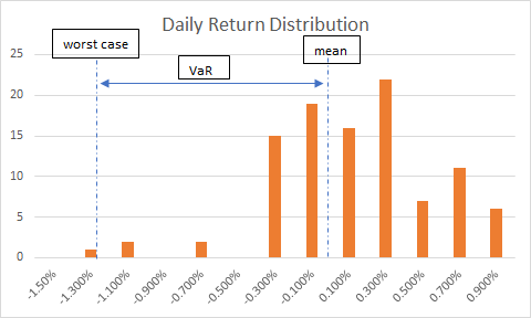
The historical method assumes that history will repeat itself from a risk perspective. The "worst" senario in the past could be used as a reference for future "worst" situation.

The calculation simply re-arrange the actual historical series of returns (or sometimes profit-and-loss), and put them in order from worst to best. Then, the α-percentile is estimated as VaR.

For example, suppose our portfolio contains only 1 stock which has a market value of US$100,000. We collected the previous 101 daily returns of the stock:

We sort the returns in ascending order:

Therefore, we have

• the next day's expected PL = 100000*(-1.3% - 1.2% + ... + 0.8%)/101 = 39.3069
• the next day's worst PL at 99% confidence level = -1.2%*100000 = -1200.
• then, 99% 1-day VaR (or sometime called "Unexpected Loss") is calculated as 39.3069 - (-1200) = 1239.3069

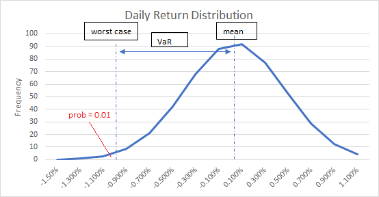
Parametric VaR

The parametric method is also called Variance-Covariance method, which assumes that stock returns are normally distributed. In other words, it only requires to estimate 2 parameters:

• expected return
• standard deviation

These 2 factors define the shape of a normal distribution curve. Using the same example above, we compute mean = 0.39307%, and standard derivation = 0.004314818 for the return series.

The corresponding inverse normal distribution at 1% is calculated to be -0.009644698, which is interpreted as the worst return at 99% confidence level. Thus, 99% 1-day VaR would be 100000*(0.39307% - (-0.009644698)) = 1003.78

We can see the VaR result is closed to the one obtained in historical method.

Backtesting VaR

The daily profits-and-losses (PL) against value-at-risk (VaR) for an actual trading portfolio is usually plotted in the following way.

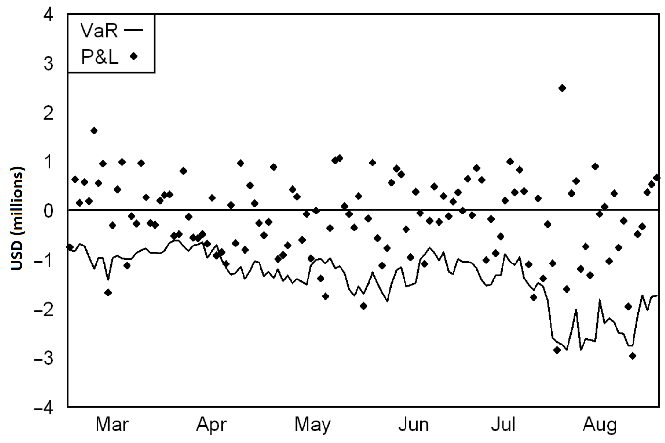
The chart summarize the portfolio's daily performance and the evolution of its market risk. It provides a simple graphical analysis of how well a VaR measure performed.

For a 95% 1-day VaR metric, we expect there are roughly 5% of the time (or 6 in a 6-month period). From the chart, we can count 10 exceedances over the six months. Does this VaR measure reasonably perform as expected???

To answer this, we can refer to some statistically testing techniques. Most of the published backtesting methodologies can be categorised into:

• Coverage tests - test whether the frequency of exceedances is consistent with the quantile of loss a VaR measure
• Distribution tests - goodness-of-fit tests applied to the overall loss distributions forecast by complete VaR measures
• Independence tests - test whether exceedances appear to be independent from one period to another

Limitation of VaR

1. The result of VaR may underestimate the actual loss.

VaR simply focuses on the manageable risks near the center of the loss distribution and ignored the tails. For example, a 99% 1-day VaR of 15% represents an expectation of losing at least 15% once every 100 days on average. For this calculation, a loss of 50% still validate the risk accessment.

2. Selection bias

For example, VaR calculated using a period of low volatility may understate the potential for risk events to occur and its magnitude. Risk may also be understated using normal distribution, which does not account for extreme events.

3. Require huge computation resource

For a global bank involving 24-hour transactions, it is already difficult to retrieve all positions from a large portfolio in a real-time basis. Let's alone to calculate the VaR result, espectially when a portfolio consists of complicated and illiquid derivatives positions where mark-to-market price is not available.

The 2008 financial crisis actually reflected these problems where VaR calculations understated the potential occurrence of risk events and the risk magnitude. It resulted in extreme leverage taken within subprime portfolios. As a result, it left institutions unable to cover billions of dollars in losses as subprime mortgage values collapsed.

Conclusion

VaR provides a systemaic and relatively simple method to quantify financial risk, but it ignores everything outside the VaR limit. In reality, loss distribution typically has fat tails. Knowing the distribution of losses beyond the VaR point is almost impossible. Risk manager should apply further analysis like Stress Testing to plan for "Excess Loss".