Introduction

The Hurst exponent, denoted as H, is a measure of the long-term memory of time series data. Originally developed to analyze hydrological data, it has gained prominence in financial markets due to its ability to characterize the behavior of asset prices. Understanding the Hurst exponent can help traders identify whether a time series exhibits trends, mean reversion, or random walk behavior, which is crucial for developing effective trading strategies.

What is the Hurst Exponent?

The Hurst exponent is defined in the range of 0 ≤ H ≤ 1

• H < 0.5: Indicates mean-reverting behavior. The series tends to revert to its mean.
• H = 0.5: Suggests a random walk (Brownian motion), indicating no long-term memory.
• H > 0.5: Implies trending behavior. The series exhibits persistence, meaning that an upward trend is likely to be followed by further upward movements.

Calculating the Hurst Exponent

One common method for estimating the Hurst exponent is the Rescaled Range (R/S) analysis. The steps are as follows:

1. Calculate the mean of the time series Y(t)
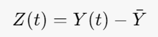
2. Calculate the deviations from the mean:


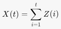
3. Calculate the cumulative deviations:


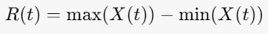
4. Calculate the range R(t):


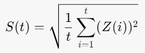
5. Calculate the standard deviation S(t) of the time series:


6. Compute the rescaled range R/S:


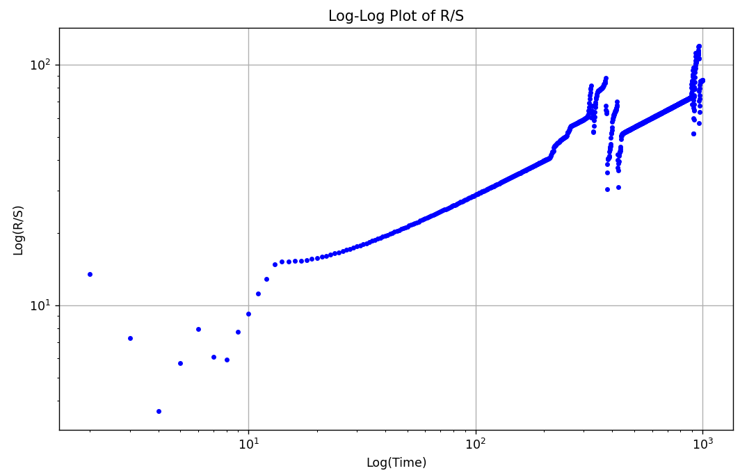
7. Repeat for various time lags t and plot log(t) vs log(R/S)


8. The slope of the line in this log-log plot gives the Hurst exponent H

Python Implementation

Here is a Python function to calculate the Hurst exponent using the R/S method

 1
 2
 3
 4
 5
 6
 7
 8
 9
10
11
12
13
14
15
16
17
18
19
20
21
22
23
24
25
26
27
28
29
30
31
32
33
34
35
36
37
38
39
40
41
42
43
44
45
46
47
48
49
50
51
52
53
54
55
56
57
58
59
60

import numpy as np
import pandas as pd
import matplotlib.pyplot as plt

def hurst_exponent(ts):
    # Calculate the mean of the time series
    N = len(ts)
    Z = ts - np.mean(ts)

    # Calculate cumulative deviations
    X = np.cumsum(Z)

    # Calculate R/S for different time lags
    T = np.arange(2, N)  # Start from 2 to avoid division by zero
    R_S = []

    for t in T:
        # Calculate range R(t)
        R = np.max(X[:t]) - np.min(X[:t])
        
        # Calculate standard deviation S(t)
        S = np.std(ts[:t])

        if S != 0:  # Prevent division by zero
            R_S.append(R / S)
        else:
            R_S.append(np.nan)  # Append NaN if S is 0

    # Fit log-log model to estimate Hurst exponent
    log_T = np.log(T)
    log_R_S = np.log(R_S)

    # Remove NaN values for fitting
    mask = ~np.isnan(log_R_S)
    H = np.polyfit(log_T[mask], log_R_S[mask], 1)[0]

    return H

# Example usage
# Generate a sample time series (e.g., simulated stock prices)
np.random.seed(42)
n = 1000
returns = np.random.normal(0, 1, n)
prices = np.exp(np.cumsum(returns))  # Simulate price series

# Calculate Hurst Exponent
H = hurst_exponent(prices)
print(f"Hurst Exponent: {H:.4f}")

# Plot R/S
T = np.arange(2, len(prices))  # Start from 2
R_S = [np.max(np.cumsum(prices[:t]) - np.min(np.cumsum(prices[:t]))) / np.std(prices[:t]) for t in T]

plt.figure(figsize=(10, 6))
plt.loglog(T, R_S, 'b.')
plt.title('Log-Log Plot of R/S')
plt.xlabel('Log(Time)')
plt.ylabel('Log(R/S)')
plt.grid()
plt.show()

Interpretation

In practice, the Hurst exponent can guide trading decisions. For instance:

• If H < 0.5: Consider employing mean-reversion strategies, such as pairs trading or statistical arbitrage.
• If H > 0.5: Trend-following strategies may be more appropriate, such as momentum trading or using moving averages.

Limitations

While the Hurst exponent is a valuable tool, it is not without limitations:

• Sensitivity to Noise: Financial time series data can be noisy, and the Hurst exponent may be affected by outliers.
• Stationarity Assumption: The method assumes that the time series is stationary, which may not hold true for all financial assets.

Conclusion

The Hurst exponent offers insightful perspectives on the behavior of financial time series. By understanding whether a market exhibits mean-reverting or trending behavior, professional traders can develop more informed and effective trading strategies. As always, it’s essential to complement the Hurst analysis with other indicators and market insights to enhance decision-making.

Feel free to experiment with the provided Python code and adapt it to your specific trading scenarios!