
Welcome to my first post! Today, we’re diving into an essential concept for traders: the Kelly Criterion. This mathematical formula helps determine the optimal size of a series of bets or investments to maximize long-term growth. Let’s explore its assumptions, application in the stock market, and provide a practical Python script to implement a trading strategy based on this criterion.
What is the Kelly Criterion?
The Kelly Criterion was developed by John L. Kelly Jr. in 1956. It provides a strategy for bet sizing in gambling and investing, aiming to maximize the expected logarithm of wealth. The formula is:
where
- f * = fraction of the capital to wager
- b = odds received on the wager (b to 1)
- p = probability of winning
- q = probability of losing (1 - p)
Assumptions of the Kelly Criterion
- Probability Estimation: The user must accurately estimate the probability of winning and losing.
- Independent Events: Each investment or bet must be independent of the others.
- Infinite Capital: The model assumes unlimited capital and continuous betting opportunities.
- Logarithmic Utility: It assumes that wealth grows exponentially, which might not hold in all market conditions.
Applying the Kelly Criterion in the Stock Market
In the stock market, the Kelly Criterion can be used to determine the optimal investment size in a particular stock or portfolio based on the expected returns and risks:
- Estimate Probabilities: Use historical data or statistical models to estimate the probability of a price increase (p) and decrease (q).
- Determine Odds: Calculate the expected return relative to the risk involved.
- Calculate the Fraction: Use the Kelly formula to determine the fraction of your capital to invest.
Assume you have a stock with:
- 70% probability of increasing in value (p = 0.7)
- 30% probability of decreasing in value (q = 0.3)
- Expected return of 20% (b = 0.2)
Using the Kelly Criterion: f * = (0.2*0.7 - 0.3) / 0.2 = -0.8
In this case, the result indicates a negative fraction, suggesting that this investment isn't favorable.
Quick Example
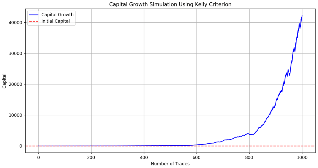
Assume our initial capital is $1. Suppose we have a trading strategy with winning rate 55%. The average win is +10% return, and the average loss is -5% return. Let's run a simulation for 1000 trades if we apply the Kelly fraction for the investment size.
1 2 3 4 5 6 7 8 9 10 11 12 13 14 15 16 17 18 19 20 21 22 23 24 25 26 27 28 29 30 31 32 33 34 35 36 37 38 39 40 41 42 43 44 45 46 47 | import numpy as np import matplotlib.pyplot as plt # Parameters np.random.seed(42) # For reproducibility num_trades = 1000 # Number of trades win_rate = 0.55 # Probability of winning avg_win = 0.1 # Average win (10% return) avg_loss = -0.05 # Average loss (-5% return) # Kelly Criterion Calculation def calculate_kelly(p, b): q = 1 - p return (b * p - q) / b # Simulate Trades def simulate_trades(num_trades, win_rate, avg_win, avg_loss): kelly_fraction = calculate_kelly(win_rate, avg_win / abs(avg_loss)) capital = 1.0 # Starting capital capital_history = [capital] for _ in range(num_trades): if np.random.rand() < win_rate: # Win capital += capital * kelly_fraction * avg_win else: # Loss capital += capital * kelly_fraction * avg_loss capital_history.append(capital) return capital_history # Run the simulation capital_history = simulate_trades(num_trades, win_rate, avg_win, avg_loss) # Plot the results plt.figure(figsize=(12, 6)) plt.plot(capital_history, label='Capital Growth', color='blue') plt.title('Capital Growth Simulation Using Kelly Criterion') plt.xlabel('Number of Trades') plt.ylabel('Capital') plt.axhline(y=1, color='red', linestyle='--', label='Initial Capital') plt.legend() plt.grid() plt.show() |
SPY Strategy Backtest Example
Wow! We got a very promising result from the example above. Let's further backtest this idea using real market data. We will apply on SPY.US
Backtest Setting
- Instrument: SPYUS
- Initial Capital: US$100,000
- Start Date: 2024-01
- End Date: 2024-07
- Data Interval: 1-day
- Short-selling: No
- Leverage: 1
Step 1. Define a function to calculate Kelly fraction
1 2 3 | def calculate_kelly(p, b): q = 1 - p return (b * p - q) / b |
Step 2. Initialize variables and get the contract size of SPY
1 2 3 4 5 6 7 8 9 10 11 12 13 14 15 16 17 18 | from AlgoAPI import AlgoAPIUtil, AlgoAPI_Backtest from datetime import datetime, timedelta class AlgoEvent: def __init__(self): self.timer = datetime(1970,1,1) self.last_close = None self.returns = [] self.numObs = 30 def start(self, mEvt): self.evt = AlgoAPI_Backtest.AlgoEvtHandler(self, mEvt) # get lot size self.instrument = mEvt['subscribeList'][0] self.contractSize = self.evt.getContractSpec(self.instrument)["contractSize"] self.evt.start() |
Step 3. Compute daily return and Kelly fraction
1 2 3 4 5 6 7 8 9 10 11 12 13 14 15 16 17 18 19 20 21 22 | def on_marketdatafeed(self, md, ab): if md.timestamp >= self.timer+timedelta(hours=24): self.timer = md.timestamp # update return series if self.last_close!=None: self.returns.append(md.lastPrice/self.last_close-1) self.last_close = md.lastPrice # keep only the recent observations if len(self.returns)>=self.numObs: self.returns = self.returns[-self.numObs:] # calculate Kelly Criterion win_rate = sum([1 for r in self.returns if r>0])/len(self.returns) avg_win = sum([r for r in self.returns if r>0])/len(self.returns) avg_loss = sum([r for r in self.returns if r<0])/len(self.returns) b = abs(avg_win/avg_loss) kelly_fraction = calculate_kelly(win_rate, b) if kelly_fraction<=0 or kelly_fraction>1: return |
Step 4. Round to the closest number of lot and open position
1 2 3 4 5 6 7 8 9 10 11 | quantity = round(ab['availableBalance']*kelly_fraction/(md.lastPrice*self.contractSize), 0) if quantity>0: order = AlgoAPIUtil.OrderObject( openclose = "open", instrument = md.instrument, buysell = 1, volume = quantity, ordertype = 0, # market order holdtime = 24*60*60 # hold for 1 day only ) self.evt.sendOrder(order) |
Full Script
1 2 3 4 5 6 7 8 9 10 11 12 13 14 15 16 17 18 19 20 21 22 23 24 25 26 27 28 29 30 31 32 33 34 35 36 37 38 39 40 41 42 43 44 45 46 47 48 49 50 51 52 53 54 55 56 57 58 59 | from AlgoAPI import AlgoAPIUtil, AlgoAPI_Backtest from datetime import datetime, timedelta def calculate_kelly(p, b): q = 1 - p return (b * p - q) / b class AlgoEvent: def __init__(self): self.timer = datetime(1970,1,1) self.last_close = None self.returns = [] self.numObs = 30 def start(self, mEvt): self.evt = AlgoAPI_Backtest.AlgoEvtHandler(self, mEvt) # get lot size self.instrument = mEvt['subscribeList'][0] self.contractSize = self.evt.getContractSpec(self.instrument)["contractSize"] self.evt.start() def on_marketdatafeed(self, md, ab): if md.timestamp >= self.timer+timedelta(hours=24): self.timer = md.timestamp # update return series if self.last_close!=None: self.returns.append(md.lastPrice/self.last_close-1) self.last_close = md.lastPrice # keep only the recent observations if len(self.returns)>=self.numObs: self.returns = self.returns[-self.numObs:] # calculate Kelly Criterion win_rate = sum([1 for r in self.returns if r>0])/len(self.returns) avg_win = sum([r for r in self.returns if r>0])/len(self.returns) avg_loss = sum([r for r in self.returns if r<0])/len(self.returns) b = abs(avg_win/avg_loss) kelly_fraction = calculate_kelly(win_rate, b) if kelly_fraction<=0 or kelly_fraction>1: return # round to the closest number of lot quantity = round(ab['availableBalance']*kelly_fraction/(md.lastPrice*self.contractSize), 0) if quantity>0: order = AlgoAPIUtil.OrderObject( openclose = "open", instrument = md.instrument, buysell = 1, volume = quantity, ordertype = 0, # market order holdtime = 24*60*60 # hold for 1 day only ) self.evt.sendOrder(order) |
Backtest Result
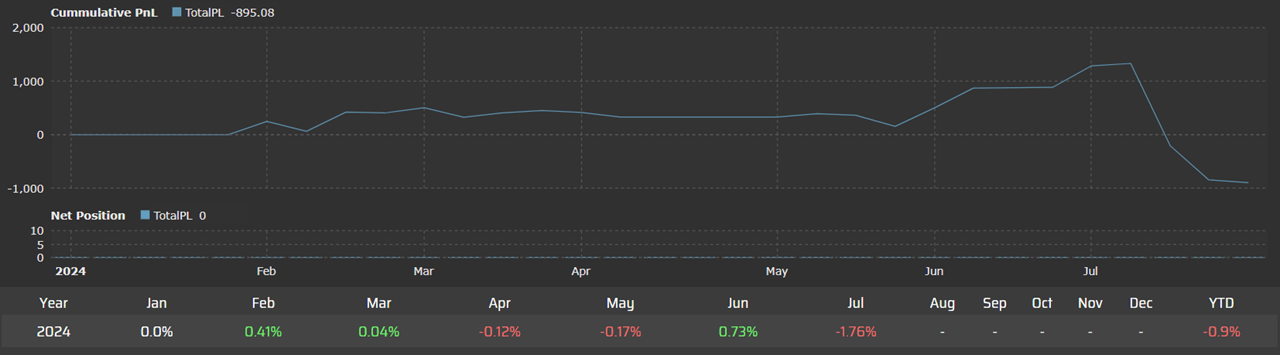
Final Thoughts
Why the performance is not as good as in the previous example???
The Kelly fraction is originally designed to apply to gambling in casino, not financial market. There are fundamental differences:
| Gambling | Investment |
|---|---|
| The risk and reward are determined. (eg. 50% win rate for flipping a coin) | The chance of winning a trade is a variable |
| Each bet has only binary outcomes which are determined. (eg. Every time when if you win, you get $10, if you loss, you loss $5) | The outcome is the investment return which is a continuous variable |
| Each bet is independent | There could be serial correlation |
Yet Kelly fraction is still a useful technique for capital management. Some modifications we can consider when applying Kelly crierion in financial market:
- For risk averse traders, we only trade at a fraction of 𝑓 ∗
- Define a take-profit and stop-loss level (eg. 20 points from entry price) so that it fixes the profit/loss amount of each trade
- Instead of applying Kelly formula directly to the original price, we can apply it to the trading signals generated from other models. It is to ensure the trades are independent
- Other research paper proposes a continous version
Like and follow me
If you find my articles inspiring, like this post and follow me here to receive my latest updates.
Enter my promote code "UYxWJS8cH1uG" for any purchase on ALGOGENE, you will automatically get 5% discount.

