
By performing the Singular Spectrum Analysis (SSA) or Singular Value Decomposition (SVD) on moving average helps improve the sensitivity of the model to pivot points and rebounces. SSA is often used to smooth out noise of univariate time-series and to study their spectral characteristics.
The aim of SSA is to decompose a time series into smaller components to better interpret its trends. SSA takes the chracteristic difference between a sliding window as the major contributing signal and ignores the rest, hence achieving the best de-noising effect.
SSA Calculation
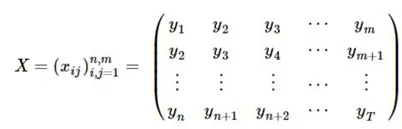
The above matrix X maps the trajectory of the x. m is the sliding window, where n = T - m + 1, We will performing SVD on the matrix X.T*X. We will be extracting a set of matrix {m} of the eigenvalues: λ1 ≥ λ2 ≥ ⋯ ≥ λm ≥ 0.
There are four steps to the calculation.
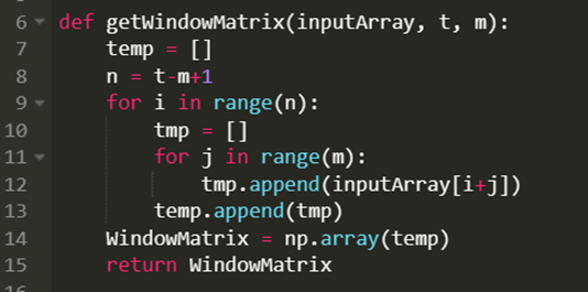
Step 1. Get window matrix
First we will have to choose an appropriate length for the slinding window where . By transforming all observed 1D time-series data into a 2D matrix, so that the trajectory matrix X = [X1,...,Xn] = (xij)n, m i,j = 1 has values X1,...,Xn, (Xi = (yi, ... yi+m-1), n = T-m+1).
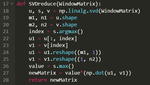
Step 2. Perform SVD
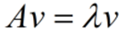
According to the Eigen decomposition theorem, v is the eigenvector and A is a square matrix.
The above can also be written as follows,
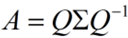
where Σ is the diagonal Matrix and Q is the orthogonal matrix.
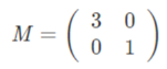
Suppose we have a matrix of M,
If we multiply the matrix by the directional vectors (x, y) the result will be as follows,
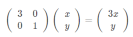
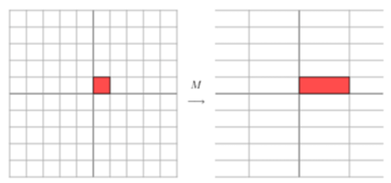
We can see a change in the directional vector (x, y) after the tranformation (multiplication). When the matrix M to be mutiplied is not symmetrical,
The directional vector changes its direction pointing to the blue arrow,
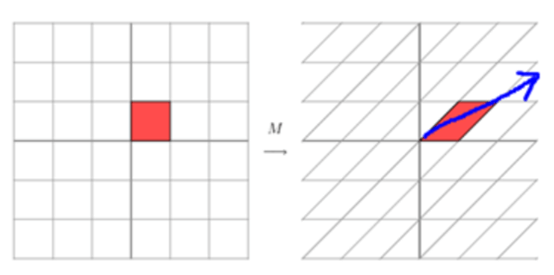
To capture a pivot point, we can use the above change in the directional vector as a signal. By performing eigen decomposition we can obtain the eigenvector and eigenvalues of the tragectory matrix. However, there are also limitations to eigen decomposition, it requires the matrix to be investigated to be a square matrix.
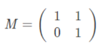
In order to combat the stated issue with the eigen decomposition theory. SVD provides a convienient solution for an NxM matrix. Take the following matrix as an example,
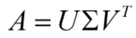
V is an NxN matrix, U is an MxM matrix and the diagonal matrix takes the shape of MxN. By performing matrix diagonalization,
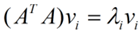
The v here corresponds to the right single-vector, where u is the left single-vector,
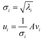
σ is the single-value which is very similar to an eigenvalue, it is rapidly decreasing, the top 10% or 1% of the sum of eigenvalues is the top 99% or above of the sum of single-values. The first single-value is extracted and used to recreate the trajectory matrix.
Step 3. Recreating the Trajectory Matrix (Time-Series)
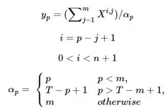
With normalization to smooth out the time series,
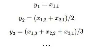
We can rebuild the matrix using the following equation,
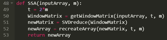
The code is as follows,
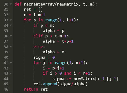
Step 4. Define the Parameters
To put it all together,
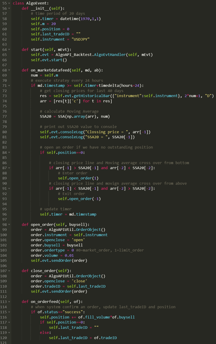
Rest of the code
Results
Backtest Settings:
- Instrument: USDJPY
- Period: 2022.10 - 2023.08
- Initial Capital: US$10,000
- Data Interval: 1-day bar
- Allow Shortsell: True
Backtest Result
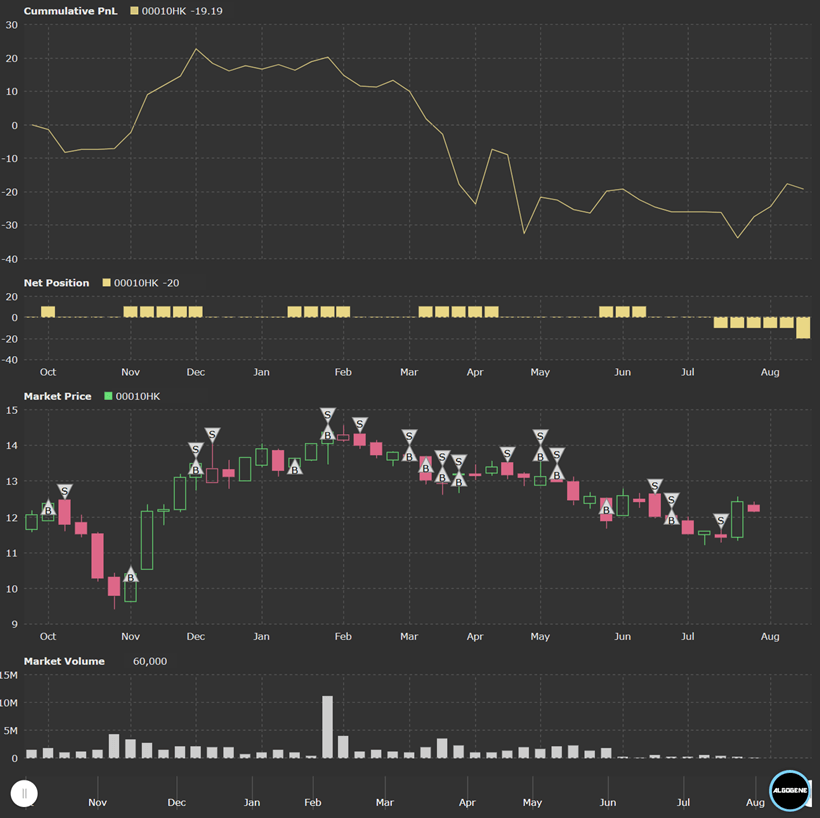
Conclusions
As we can see the strategy doesn’t perform too well, this could be due to a few different factors:
- The sliding window period m is set to 20 days, this could be further adjusted to cater to the specific asset’s volatility
- A stop loss level can be deployed to prevent excessive downside

