
What is an Autoregressive Model?
An autoregressive (AR) model predicts future behavior based on past results. It is used for forecasting when there is some correlation between values in a time series and the values that precede and succeed them. You only use past data to model the behavior, hence the name autoregressive (the Greek prefix auto means 'self'). The process is basically a linear regression of the data in the current series against one or more past values in the same series.
In an AR model, the value of the outcome variable (Y) at some point t in time, like a 'regular' linear regression, directly related to the predictor variable (X). Where simple linear regression and AR models differ is that Y is dependent on X and previous values for Y.
The AR process is an example of a stochastic process, which have degrees of uncertainty or randomness built in. The randomness means that you might be able to predict future trends pretty well with past data, but you’re never going to get 100% accuracy.
AR models are also called conditional models, Markov models, or transition models.
AR(p) Models
An AR(p) model is an autoregressive model where specific lagged values of yt are used as predictor variables. Lags are where results from one time period affect following periods.
The value for 'p' is called the order. For example, an AR(1) would be a 'first order autoregressive process.' The outcome variable in a first order AR process at some point in time t is related only to time periods that are one period apart (i.e. the value of the variable at t – 1). A second or third order AR process would be related to data two or three periods apart.
The AR(p) model is defined by the equation:
Where:
- yt-1, yt-2…yt-p are the past series values (lags),
- εt is random term (or called white noise),
- and δ is defined by the following equation:
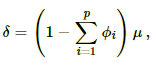
where μ is the process mean
Parameter Estimation
From the equation, all {yt} terms are already observable and known to us. What we want to get is the coefficient terms, i.e. δ, φ1, φ2, ...
(A) Least Squares Regression
One of the estimation methods is to formulate as a least squares regression problem, basing prediction of values of yt on the p previous values of the same series. A general multiple linear regression is written as:
Then, we try to minimize the sum of square error:
L(β) := Σ(εt2)
= ||Xβ - Y||2
= (Xβ - Y)T(Xβ - Y)
= YTY - YTXβ - βTXTY + βTXTXβ
As it is a convex function, the optimal solution lies at gradient zero. So we firstly take a partial derivative.
∂L(β)/∂β = ∂ (YTY - YTXβ - βTXTY + βTXTXβ) / ∂β
= -2XTY + 2XTXβ
Set this gradient to zero, we get the optimal parameters.
β = (XTX)-1XTY
Example
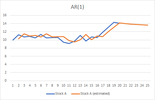
Suppose we collected the previous 20 daily closing price of stock A.
10, 11.3, 10.71, 10.87, 10.48, 11.36, 10.49, 10.57, 10.58, 9.42, 9.11, 9.75, 11.14, 9.72, 10.73, 10.57, 11.91, 13.09, 14.34, 14.09
Now, we want to use an AR(1) model (i.e. yt = δ + φ1yt-1 + εt), to explain this series.
Using the least square estimation method above, we obtained δ, φ1 = 1.319141067 and 0.898255165 respectively.
Then, we can calculate the expected value of y at time t given that we know the information for t-1, i.e. E(yt|yt-1)
| Seq | yt | Estimated yt |
|---|---|---|
| 1 | 10 | - |
| 2 | 11.3 | 10.3016927176918 |
| 3 | 10.71 | 11.4694244322527 |
| 4 | 10.87 | 10.939453884875 |
| 5 | 10.48 | 11.0831747112825 |
| 6 | 11.36 | 10.7328551969143 |
| 7 | 10.49 | 11.5233197421555 |
| 8 | 10.57 | 10.7418377485647 |
| 9 | 10.58 | 10.8136981617685 |
| 10 | 9.42 | 10.8226807134189 |
| 11 | 9.11 | 9.78070472196458 |
| 12 | 9.75 | 9.50224562080005 |
| 13 | 11.14 | 10.07712892643 |
| 14 | 9.72 | 11.3257036058452 |
| 15 | 10.73 | 10.0501812714786 |
| 16 | 10.57 | 10.957418988176 |
| 17 | 11.91 | 10.8136981617685 |
| 18 | 13.09 | 12.0173600829313 |
| 19 | 14.34 | 13.0773011776866 |
| 20 | 14.09 | 14.2001201339952 |
Moreover, we can base on the formula to further iteratate and forecast the next stock prices.
| Seq | yt | Estimated yt |
|---|---|---|
| 21 | - | 13.9755563427335 |
| 22 | - | 13.8727567364869 |
| 23 | - | 13.7804164592112 |
| 24 | - | 13.6974713282064 |
| 25 | - | 13.6229654358659 |
Now, you understand the statistical theory behide an Auto-Regressive model. Let's further go to the next post to see how to implement as a trading strategy!